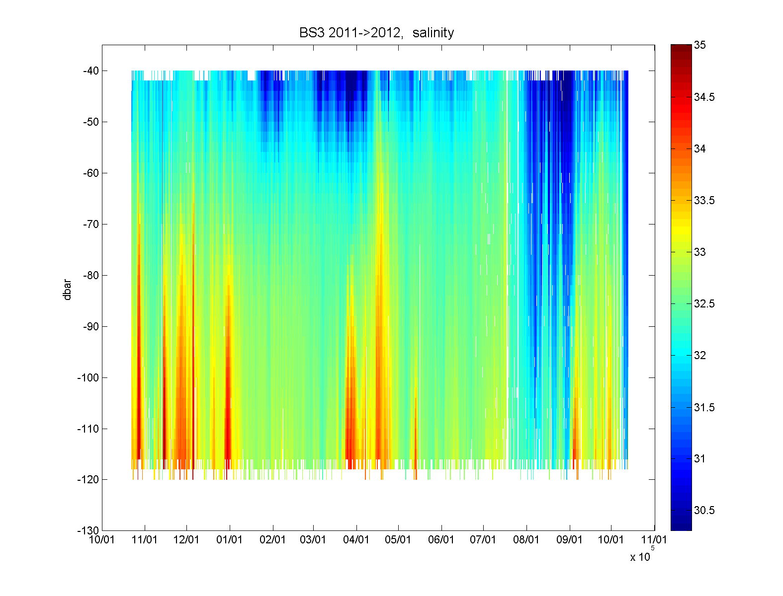
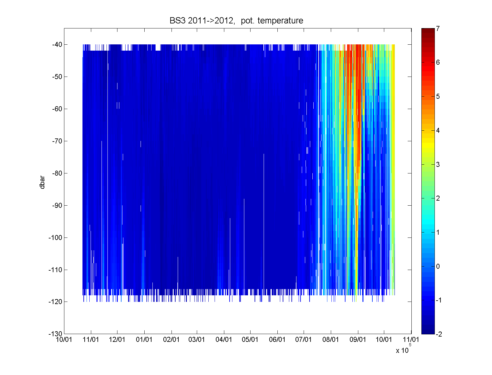
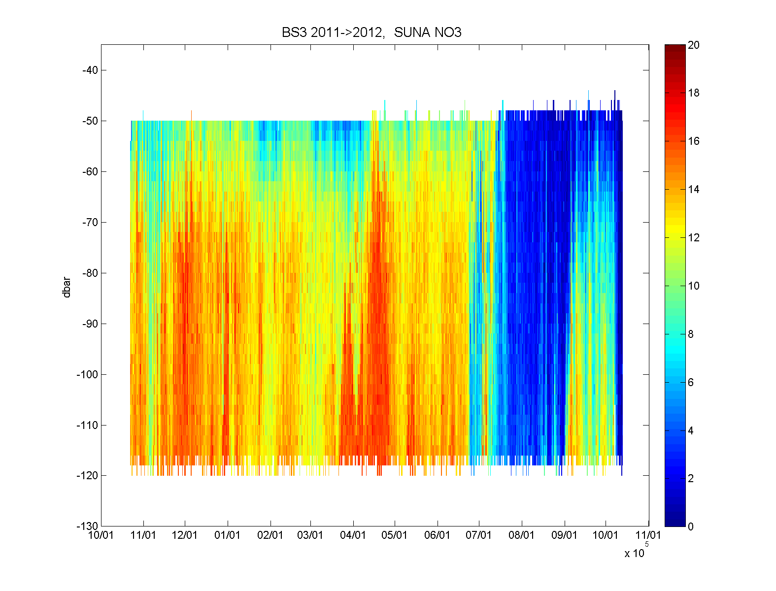
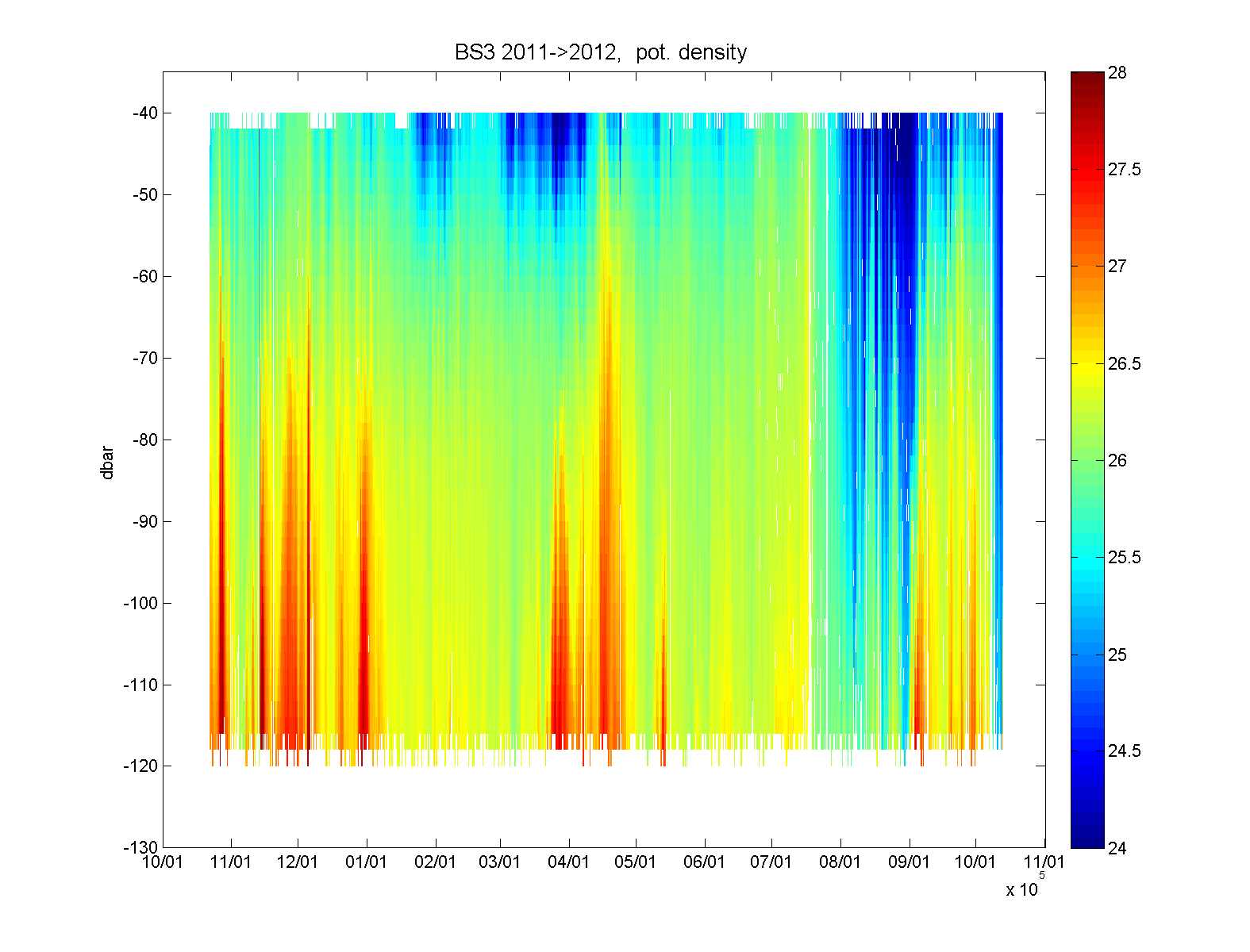
Deployment 2011 to 2012:
Coastal Moored Profiler (CMP)

Deployment summary: Duration: Oct 22, 2011 to Oct 12, 2012 Location: 71 23.645 N, 152 2.908 W, in 146.6m of water Variables measured: pressure, temperature, conductivity, O2, pH, fluorescence, backscatter,      and nitrate Sensor information: CMP is a WHOI-developed instrument similar to the McLane MMP.     onboard CTD: RBR model RBR XRX-620 with SUNA optical nitrate sensor Instrument settings: output 1Hz data Calibration: comparison to microcat located below CMP bottom stop; see cal_info; Processed data: matlab files bs3_cmp_201112_edt_pf.mat with CTD data in Paula Fratantoni's      original format, and bs3_cmp_201112_edt_fb.mat for Paula's format plus additions by fbahr.      The SUNA data are found in SUNA_binned.mat.

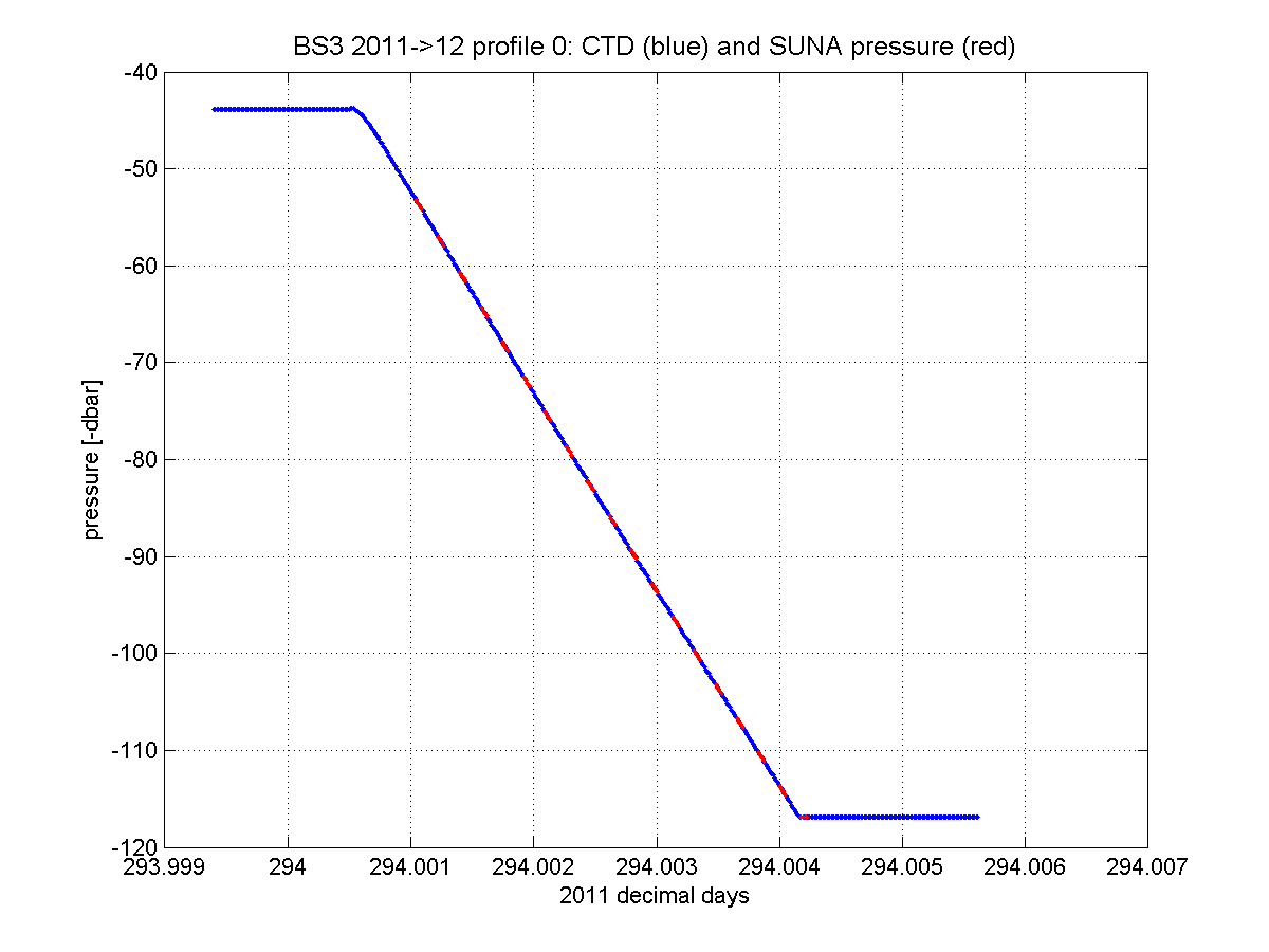
Instrument setup and recovery: The instrument was provided by Terry Hammar's shop at WHOI. Onboard the Healy, the instrument was programmed by Frank Bahr; see the programming capture for details. The mooring was recovered on Oct. 13, 2012, close to 00:00 GMT. The instrument collected two more "profiles" on deck before being shut down, confirming the 10 dbar atmospheric pressure offset. On the 20th, I connected to the CMP for a system check, indicating that the CMP clock was fast by 1 minute 7 seconds. Data processing: After retrieving the memory card from the CMP, the data were copied onto a laptop hard drive and converted from the manufacturer's format to ascii "C", "E", and "S" files using McLane's UnPacker-2.01.26.exe. From here on, software developed by John Toole and Paula Fratantoni (WHOI) was employed, with some additions and modifications by Frank Bahr. When reading in the CTD data, pressure was adjusted by 10dbar to remove a nominal atmospheric pressure of 1000 mbar. Initial coarse editing removed extreme data spikes that excluded threshold settings for pressure, temperature, and conductivity. Data from the stationary periods prior to and following the CMP travel along the mooring were removed. More careful spike editing via visual tools was employed, in particular to search for smaller spikes from conductivty, before time-filtering the data to match the temporal responses of the temperature and conductivity sensors. None were found for this deployment. Upon closer inspection, we learned that the CMP's RBR CTD had been programmed to collected 1Hz averages, rather than 6Hz data. Conductivity was lagged versus temperature and pressure to remove salinity spikes. The best lag was identified visually as one that removed or limited density inversions at sharp vertical temperature/conductivity steps. For this CMP record, the best lag was determined to be mostly 1 for the down profiles and mostly 0 for the up profiles. The resulting dataset was then averaged into 2-dbar pressure bins. Additional editing on the 2-dbar averages with Paula's elaborate tools flagged density inversions exceeding 0.005 kg/m^3, which were then visually inspected and mostly eliminated (set to NaN). Presumably because of the averaging by the CTD before output, this dataset included a higher than usual number of small inversion, and I relaxed the visual editing to leave "benign" cases in place. The final data are presented here in two matlab .mat files. One, named ".._pf.mat", comes from Paula Fratantoni's programs without modifications. The main difference between it and the second, named ".._fb.mat", is that the "fb" format may include profiles of NaN's to represent CMP profiles that were edited out entirely, typically because the CMP got stuck at one of the stops. However, this dataset did not include such gaps. SUNA notes: The SUNA data were available for only every other profile, i.e., for even profile numbers starting with zero. The SUNA (S*.TXT) files for odd numbered profile were empty. Thus, we collected dive profiles every 12 hours. The collected data consisted of a time series of groups that contained one "dark" reading (no nitrate) followed by four "light" readings and a small time gap . The dark readings coincided with the CMP's stopgap lines in the "E*.txt" files, which allowed us to match SUNA time (relative to instrument startup) to CTD pressure. The SUNA required a roughly 150 second warm-up period, which resulted in some data loss over the early portion of the profiles. The SUNA data were also averaged into 2-dbar pressure bins, using the same gridding as for the CTD. Because of the small time gaps between the dark/light reading groups, however, some vertical bins within a profile remained empty. These "interior gaps" were interpolated over. Both these interpolated profiles and the binned data with gaps, as well as the original pressure/time series, were saved for the final .mat file. A text variable "readme" further describes the data format. Details on the CTD and SUNA processing steps can be found in my processing log.