
Deployment 2009 to 2010:
Arctic Winch (AW)
final data
Arctic Winch (AW)
final data
 |
 |
|
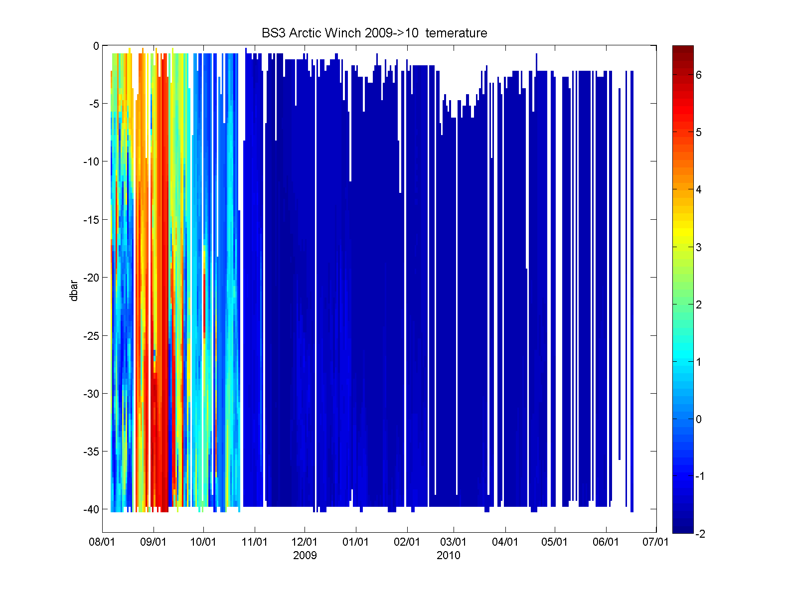
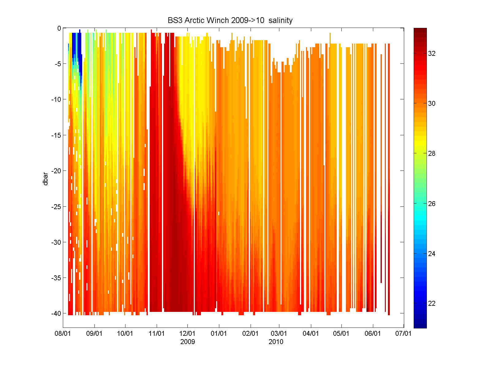
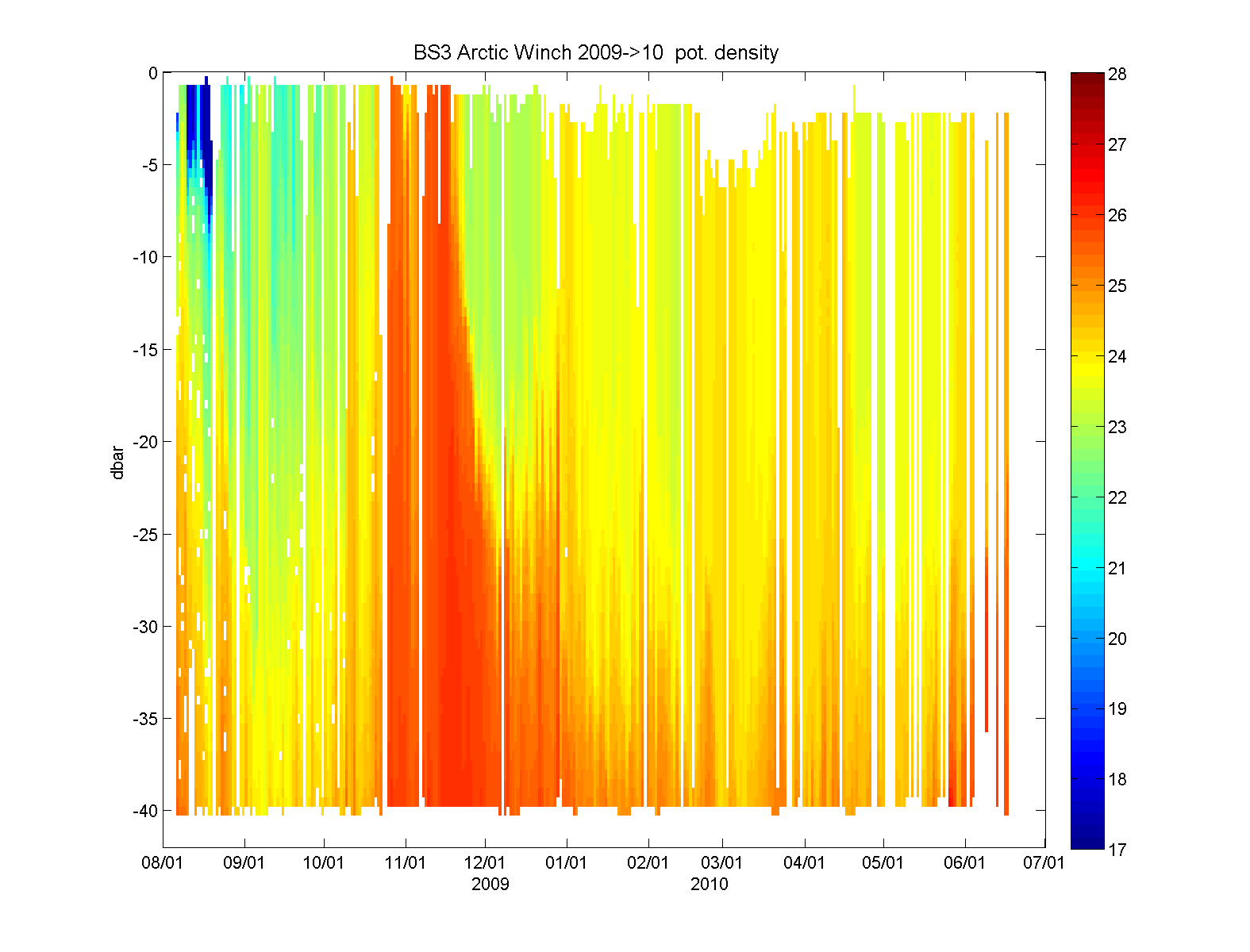
Deployment summary: Duration: Aug 4, 2009 to June 17, 2010 Location: BS3 mooring site Variables measured: pressure, temperature, conductivity, fluorescence, turbidity Sensor information: The Arctic Winch is a WHOI-developed instrument platform. For this deployment, it was equipped with an RBR CTD. Instrument settings: output 6 Hz data Calibration: comparison to nearby calibrated SEaBird SBE37 microcat Processed data: contained in the matlab files aw_bs3_200910_final.mat. The file format is described here. |
|
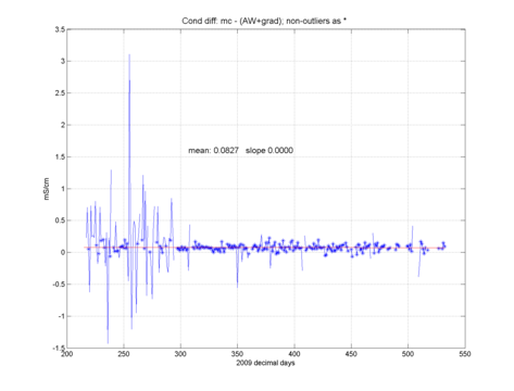
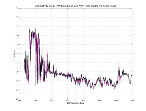
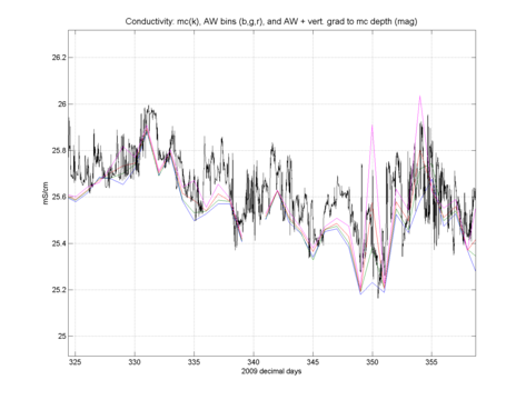
Data processing: Processing steps include: - raw time series de-spiking; - conversion of temperature/conductivity to salinity and density; - lagging of T/C relation to reduce spiking and inversions - pressure binning into standard profiles. - removal of remaining density inversions - conductivity calibration - A/D sensor voltage -> engineering data conversion Raw Data De-spiking Working on previous year's data, I spent some effort on de-spiking algorithms, eventually settling on acomparison of consecutive time series segments to a second-order fit. Outliers were identified as exceeding n standard deviations. A minimum outlier size was set to avoid editing of good points during very low variability segments. After some experimenting, I selected a subset size of 50 points, and a spike threshold of 2 std. I set a minimum spike size of 1 dbar, 0.1 deg C, and 0.5 conductivity units. Lateron, I found that basic range editing worked well as a first step, excluding points beyond simple limits of -10 to 200 dbar, -5 to 15 deg C, and 15 to 50 conductivity units, respectively. As it turned out, spiking was not much of an issue; it was mainly observed in one of the early datasets I had worked with. Salinity Derivation The Arctic winch CTD rests at depth, then ascents to the surface once a day. I split the daily profile into up (ascent) and down (descent) profiles, with the latter quite clearly providing more realistic data. The physical reason is presumably the CTD location below the float. Salinity and density were derived for several lags of temperature versus conductivity (-3 to +2 scans). A best lag was selected based on visual inspection of the down profiles. For BS3 2009-2010, it was -2 scans; it had been 0 for earlier RBR datasets or +1 for earlier FSI CTD datasets.) Pressure Binning The down cast was pressure binned using a bin size of 0.5 decibar. The bin center depth ranged from 0.25 to 79.75 dbar, though the deepest bin depth with good data was 39.75 dbar. Editing of Pressure-binned Profiles The binned profiles were examined for glitches, identified primarily by vertical density inversions. A subset of profiles - I used 10 here - were displayed in various forms: as profiles against a backdrop of the complete dataset, as TS diagrams, as well as staggered profiles of the subset. With the unducted, unpumped RBR CTD, a mismatch of temperature and conductivity to derive salinity and thus density was the primary reason for significant density inversion. They occurred primarily during the first 20% of the time series, and were manually edited out, thus leaving the "holes" in the above pcolor plots of S and sigma but not T. Conductivity Calibration The conductivity sensor calibration was checked against the post-cruise calibrated record of the microcat mounted onto the same top float of the mooring. Their vertical separation was about 1m, as shown below.  Selecting only the "quiet" periods of the record, the lowest bins of the Arctic Winch data indicated a small vertical conductivity gradient near the mooring float. We constracted a deep Arctic Winch conductivity record by averaging the three deepest bins with good data, centered on 38.25, 38.75, and 39.25 dbar, and projected it down to the microcat depth using the average vertical conductivity gradient. Microcat conductivity (black), the three deepest Arctic Winch bins, as well as the constructed deep record (magenta) are shown below for the whole time series (left) as well as for a detail from the "quiet" period (right). |
 |
 |
|
Lastly, the microcat conductivity was interpolated onto Arctic Winch profile times, |